Ultimate Ggplot Cheat Sheet: Your Go-To Guide For Mastering Data Visualization

So listen up, data enthusiasts! If you've ever found yourself scratching your head while trying to create stunning visualizations in R, you're definitely not alone. ggplot2 is one of the most powerful tools out there for creating beautiful charts and graphs, but let's be real—it can feel overwhelming at first. That’s why we’ve put together this ultimate ggplot cheat sheet to help you level up your data game. Whether you’re a beginner or an experienced coder, this guide is packed with tips, tricks, and shortcuts that will make your life easier. So grab your coffee and let’s dive in!

Data visualization is no longer just a nice-to-have skill; it’s a must-have. And ggplot2? It’s like the Swiss Army knife of data viz tools. But if you’re anything like me, you probably spend way too much time Googling the same commands over and over again. That’s why having a solid cheat sheet can save you hours of frustration. Think of this as your personal assistant for all things ggplot.

In this article, we’ll break down everything you need to know about ggplot2, from the basics to advanced techniques. We’ll cover how to create different types of plots, customize themes, add layers, and more. By the end of this, you’ll be slinging ggplot code like a pro. Let’s get started, shall we?

• Young Ted Danson The Early Years Of A Beloved Icon
• Andy Griffith Cast The Heartwarming Show That Defined A Generation

Table of Contents:

• Introduction to ggplot
• Basic Syntax and Structure
• Common Types of Plots
• Customizing Your Plots
• Adding Layers to Your Plots
• Themes and Styling
• Data Manipulation with ggplot
• Tips and Tricks for ggplot
• Best Practices for Data Viz
• Useful Resources for ggplot

Introduction to ggplot

Alright, let’s start with the basics. ggplot2 is an R package created by Hadley Wickham that implements the Grammar of Graphics. What does that mean? Well, it means that instead of thinking of a plot as a single object, you build it up layer by layer. This gives you incredible flexibility and control over every aspect of your visualization.

One of the coolest things about ggplot is how intuitive it is once you get the hang of it. You define your data, specify the aesthetic mappings (like x and y axes), and then add layers to build your plot. It’s like building a sandwich—start with the bread, add your ingredients, and voilà!

• 71 Inches To Feet A Simple Guide To Mastering This Conversion
• Ronald Fenty The Man Behind The Music And Fashion Empire

But let’s be honest, remembering all the commands and options can be tough. That’s where our ggplot cheat sheet comes in. It’s like having a cheat code for data visualization.

Basic Syntax and Structure

Before we jump into the fancy stuff, let’s talk about the foundation of ggplot. The basic syntax looks something like this:

ggplot(data = your_data, mapping = aes(x = x_var, y = y_var)) + geom_point()

Here’s what’s going on:

• ggplot(): This is where you set up your plot. You pass in your dataset and define the aesthetic mappings.
• aes(): This is where you specify which variables go on the x and y axes, as well as other aesthetics like color, size, and shape.
• geom_*: These are the layers that actually create the visual elements of your plot. For example, geom_point() creates a scatter plot, geom_line() creates a line plot, and so on.

Simple, right? But don’t worry if it doesn’t click right away. We’ll go over plenty of examples to help it sink in.

Understanding Aesthetic Mappings

Aesthetic mappings are basically how you map variables in your data to visual properties of the plot. Think of it like this: you’re telling ggplot which column in your dataset corresponds to the x-axis, which one goes on the y-axis, and what colors or shapes to use.

Here’s a quick breakdown of common aesthetic mappings:

• x: Maps a variable to the x-axis.
• y: Maps a variable to the y-axis.
• color: Maps a variable to the color of points or lines.
• size: Maps a variable to the size of points or lines.
• shape: Maps a variable to the shape of points.

For example, if you wanted to create a scatter plot where the color of the points corresponds to a categorical variable, you’d do something like this:

ggplot(data = your_data, mapping = aes(x = x_var, y = y_var, color = category)) + geom_point()

Common Types of Plots

Now that we’ve covered the basics, let’s talk about some of the most common types of plots you can create with ggplot. Whether you’re working with continuous or categorical data, ggplot has got you covered.

Scatter Plots

Scatter plots are perfect for visualizing the relationship between two continuous variables. Here’s how you create one:

ggplot(data = your_data, mapping = aes(x = x_var, y = y_var)) + geom_point()

And if you want to add a trend line to show the correlation, you can use geom_smooth():

ggplot(data = your_data, mapping = aes(x = x_var, y = y_var)) + geom_point() + geom_smooth(method ="lm")

Bar Charts

Bar charts are great for comparing categories. To create a basic bar chart, you’d do something like this:

ggplot(data = your_data, mapping = aes(x = category, y = value)) + geom_bar(stat ="identity")

If you want to stack the bars, you can add the fill aesthetic:

ggplot(data = your_data, mapping = aes(x = category, y = value, fill = subgroup)) + geom_bar(stat ="identity", position ="stack")

Line Charts

Line charts are ideal for showing trends over time. Here’s how you create one:

ggplot(data = your_data, mapping = aes(x = time, y = value)) + geom_line()

And if you want to add multiple lines for different categories, you can use the color aesthetic:

ggplot(data = your_data, mapping = aes(x = time, y = value, color = category)) + geom_line()

Customizing Your Plots

One of the things that makes ggplot so powerful is how customizable it is. You can tweak every aspect of your plot to make it look exactly how you want.

Changing Axis Labels and Titles

By default, ggplot uses the variable names as axis labels. But you can change them to make your plot more readable:

ggplot(data = your_data, mapping = aes(x = x_var, y = y_var)) + geom_point() + labs(x ="X-Axis Label", y ="Y-Axis Label", title ="Your Title")

Adjusting Colors and Themes

ggplot comes with a bunch of built-in themes that you can use to change the overall look of your plot. For example, theme_minimal() gives you a clean, minimalist design:

ggplot(data = your_data, mapping = aes(x = x_var, y = y_var)) + geom_point() + theme_minimal()

You can also customize individual elements of the theme, like the background color or font size:

ggplot(data = your_data, mapping = aes(x = x_var, y = y_var)) + geom_point() + theme(panel.background = element_rect(fill ="lightblue"), axis.text = element_text(size = 12))

Adding Layers to Your Plots

Remember how I said ggplot builds plots layer by layer? This is where things get really fun. You can add as many layers as you want to create complex, multi-faceted visualizations.

For example, you might want to add a trend line to your scatter plot, or overlay a histogram on top of a density plot. Here’s how you do it:

ggplot(data = your_data, mapping = aes(x = x_var, y = y_var)) + geom_point() + geom_smooth(method ="lm")

Or:

ggplot(data = your_data, mapping = aes(x = x_var)) + geom_histogram() + geom_density()

Themes and Styling

Themes are one of the coolest features of ggplot. They let you change the overall look and feel of your plot with just a few lines of code. Whether you prefer a clean, minimalist design or something more eye-catching, there’s a theme for you.

Built-In Themes

Here are some of the most popular built-in themes:

• theme_gray(): The default theme with a gray background.
• theme_minimal(): A clean, minimalist design.
• theme_light(): A lighter version of theme_gray().
• theme_void(): A blank canvas, great for custom designs.

Customizing Themes

But why stop at the built-in themes? You can customize every aspect of the theme to make your plot truly unique. For example, you might want to change the font, adjust the margins, or add a grid:

ggplot(data = your_data, mapping = aes(x = x_var, y = y_var)) + geom_point() + theme(text = element_text(family ="Arial", size = 14), panel.grid.major = element_line(color ="gray"))

Data Manipulation with ggplot

Sometimes your data isn’t in the exact format you need for ggplot. That’s where data manipulation comes in. Using packages like dplyr and tidyr, you can clean and transform your data before passing it to ggplot.

Filtering Data

Let’s say you only want to plot data from a specific category. You can use the filter() function from dplyr:

library(dplyr)

filtered_data % filter(category =="A")

ggplot(data = filtered_data, mapping = aes(x = x_var, y = y_var)) + geom_point()

Reshaping Data

Or maybe your data is in wide format and you need it in long format. That’s where tidyr comes in:

library(tidyr)

long_data % pivot_longer(cols = c(var1, var2), names_to ="variable", values_to ="value")

ggplot(data = long_data, mapping = aes(x = variable, y = value)) + geom_bar(stat ="identity")

Tips and Tricks for ggplot

Here are a few tips and tricks to take your ggplot skills to the next level:

• Use facets: If you have multiple categories, you can use facet_wrap() or facet_grid() to create small multiples of your plot.
• Label points: Use geom_text() or geom_label() to add labels to your points.
• Experiment with scales: ggplot has tons of options for scaling your axes, like scale_x_log10() for log transformations.

Best Practices for Data Viz

While ggplot gives you a lot of freedom,

• Cps Rapid Identity The Gamechanger In Modern Authentication
• Yoo Jungii The Rising Star Whorsquos Capturing Hearts Worldwide

Details

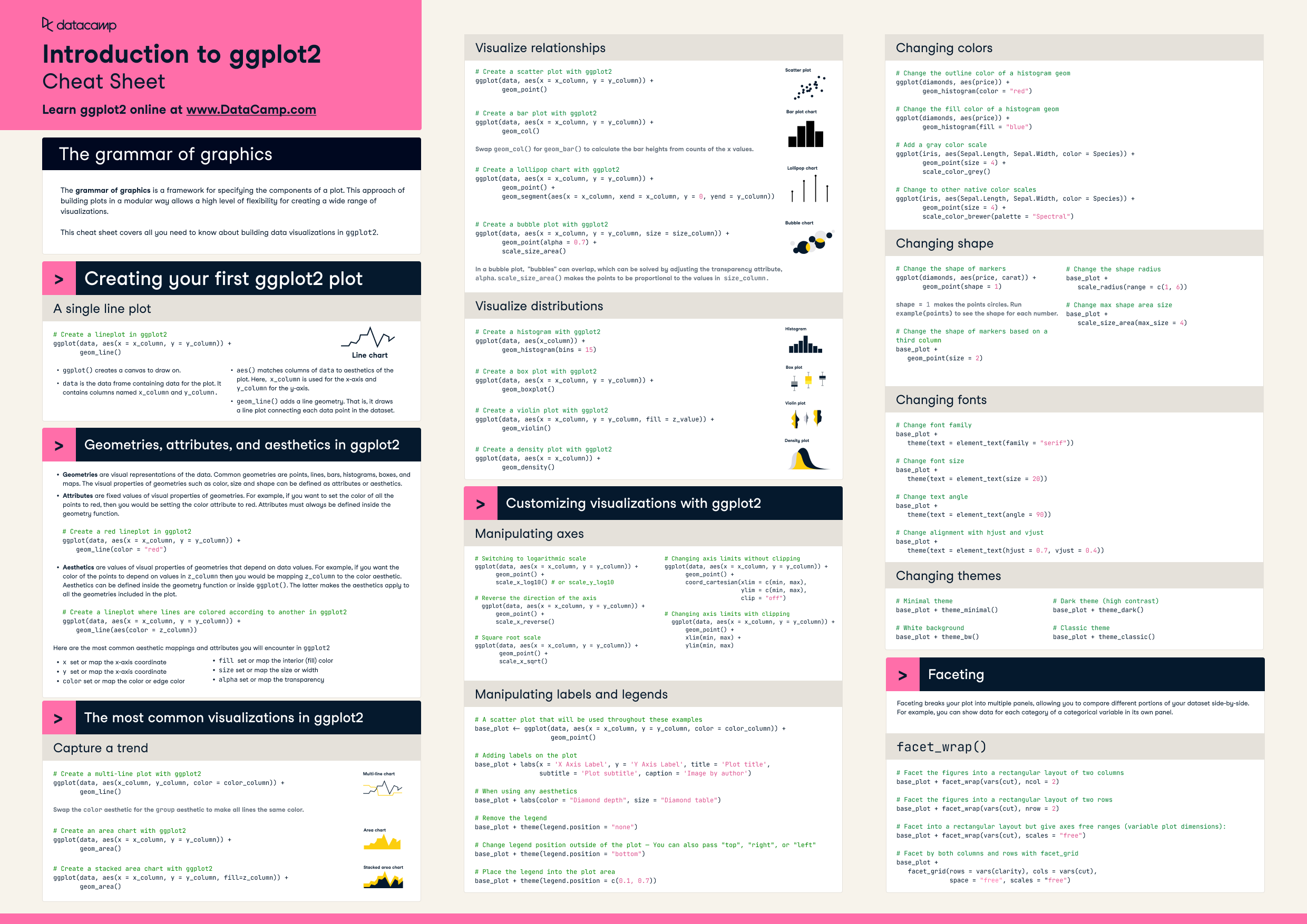
ggplot2 Cheat Sheet DataCamp

Details

Ggplot2 Cheat Sheet R Ggplot2 Cheatsheet 2 1 Eroppa

Details

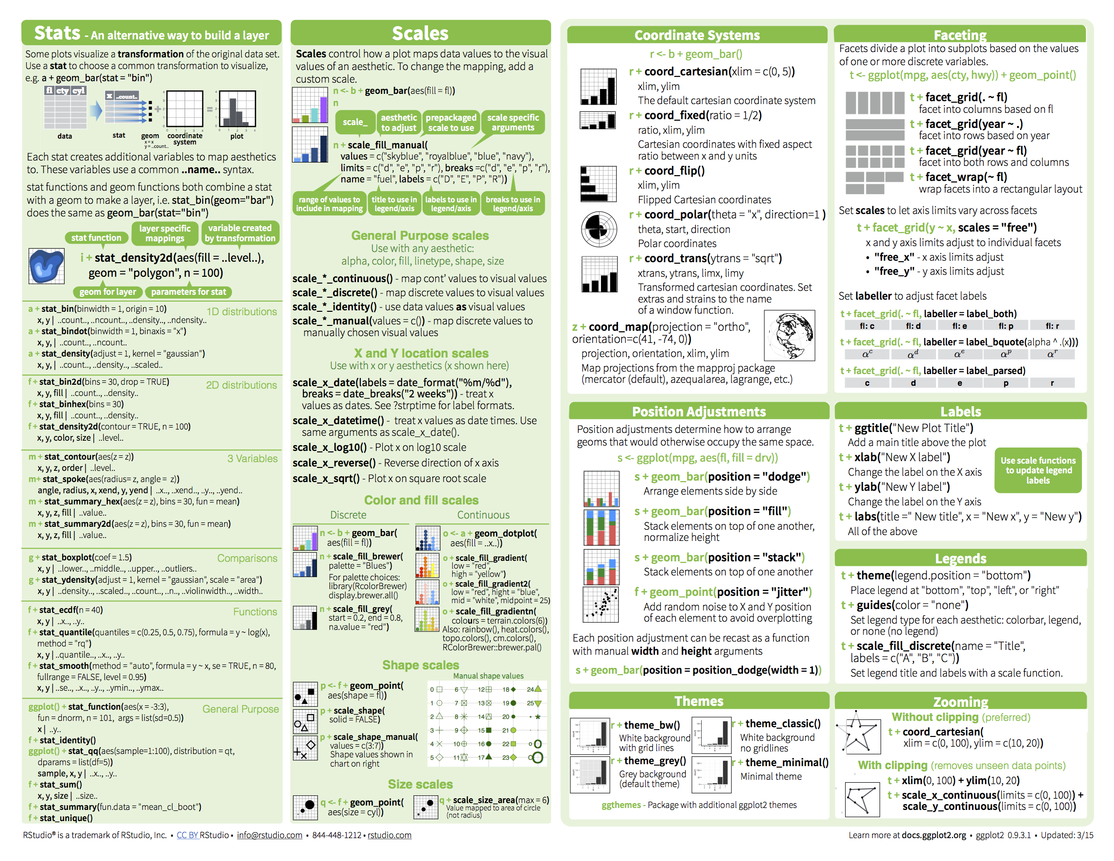
Ggplot2 Cheatsheet Info Vrogue